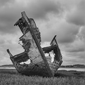
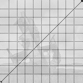
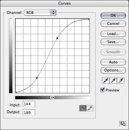
So far, we’ve used the Curves tool to adjust the white point, black point and midtones of an image, but this is nothing that we couldn’t have achieved with the Levels tool; using the black, point white point and mid-tone sliders. With the Curves tool we have much more flexibility in how we adjust the tonal range of an image, not least because you can add an additional 14 control points to the Curve, bringing the total number of control points to 16. You can add these simply by clicking the Curve, and once they’re added they can be repositioned anywhere within the grid.

One of the most useful Curves is what’s typically referred to as an S-Curve (see opposite). As you can see, two control points have been added to this Curve and it forms the approximate shape of the letter ‘S’. The upper control point lightens the lighter parts of the image while the lower point darkens the shadow areas. One thing you should note, as mentioned in the previous section, is that the steeper the Curve the greater the increase in contrast. This can be illustrated by reference to the images we used in the previous section to introduce the Curves tool, where we demonstrated that a flattened Curve would compress the tonal range while a steeper one would expand it.

If we return to those images again, we can see the difference that an S-Curve can make:

original image show curve • show histogram

expanded tonal range show curve • show histogram

expanded tonal range + S-Curve show curve • show histogram

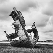
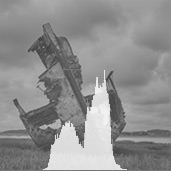
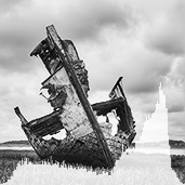
In this example the introduction of a relatively mild S-Curve has greatly improved the image: the prow of the boat is more noticeable and the boat is much more clearly delineated from the sky.

Because the original image had a restricted tonal range – from a value of 60 to 200 (see the technical note on page one if you need a reminder about what these numbers mean) – we could apply a straight-line Curve to remap the black and white points prior to introducing the S-Curve. This, however, is something you should avoid when you have an image with a more distributed tonal range.

Consider the following example:

original image show histogram

‘straight-line’ Curve show curve • show histogram

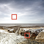
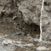
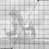
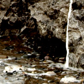
At first glance the second image, with the application of a ‘straight-line’ Curve, looks considerably improved (and the same result could have been achieved with the Levels tool). But when we look at the histogram we can see that there are problems with this image; i.e. the histogram is bunched up against both ends. What this indicates is that some of the shadow and highlight areas of the image are now ‘clipped’. In the shadow areas the darker sections of the image (pixels with an original value of 73 or less) have become black; i.e. remapped to zero, and in the highlight areas any pixel with an original value of 200 or above has been remapped to 255 (white). Again, take a look at the technical note on page one if you’re not entirely clear about what these numbers represent.

At such a small resolution this doesn’t seem particularly problematic, but when reproduced on a larger scale, when printed for example, these clipped areas are much more noticeable. This is illustrated below:

areas with clipping

original shadow detail show clipping

original highlight detail show clipping

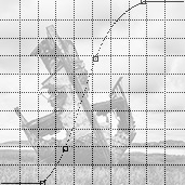
To avoid this problem we simply need to apply an S-Curve without altering the white and black points:

original image + histogram remove histogram

‘gentle’ S-Curve show curve • show histogram

‘stronger’ S-Curve show curve • show histogram

As you can see, both the ‘gentle’ and ‘stronger’ S-Curves are a big improvement on the original and, as the histograms demonstrate, both avoid clipping the shadow and highlight details, yet both stretch the distribution of tones within the image.

With experience, constructing a Curve to enhance an image is something you can do intuitively (at least most of the time), but there are a couple of techniques you can use to help you make the most of your images and the Curves tool. The first of these – using the eyedropper tool to evaluate an image prior to constructing your curve – is discussed in the next section of this tutorial.

David J. Nightingale © 2003–18 • all rights reserved

<<< previous page • next page >>>